笔记|统计学习方法:逻辑斯蒂回归与最大熵
基本介绍
逻辑斯蒂回归(Logistic Regression),虽然被称为回归,其实是一种解决分类问题的算法。 LR模型是在线性模型的基础上,使用sigmoid激励函数,将线性模型的结果压缩到
回归模型:
其中wx线性函数:
逻辑斯蒂分布
对逻辑斯蒂分布的说明如下:
分布函数
密度函数
其中,
图像:
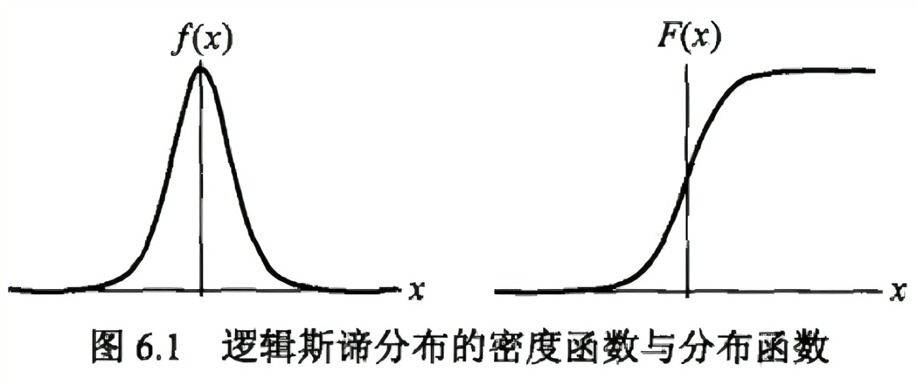
且分布函数以点
逻辑斯蒂模型
逻辑斯谛回归模型是由以下条件概率分布表示的分类模型。逻辑斯谛回归模型可以用于二类或多类分类。
逻辑斯谛回归模型源自逻辑斯谛分布,其分布函数
最大熵模型
最大熵模型是由以下条件概率分布表示的分类模型。最大熵模型也可以用于二类或多类分类。
其中,
最大熵模型可以由最大熵原理推导得出。最大熵原理是概率模型学习或估计的一个准则。最大熵原理认为在所有可能的概率模型(分布)的集合中,熵最大的模型是最好的模型。
最大熵原理应用到分类模型的学习中,有以下约束最优化问题:
求解此最优化问题的对偶问题得到最大熵模型。
总结
逻辑斯谛回归模型与最大熵模型都属于对数线性模型。
逻辑斯谛回归模型及最大熵模型学习一般采用极大似然估计,或正则化的极大似然估计。逻辑斯谛回归模型及最大熵模型学习可以形式化为无约束最优化问题。求解该最优化问题的算法有改进的迭代尺度法、梯度下降法、拟牛顿法。
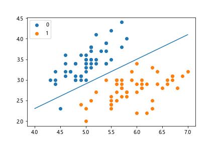
例子1-逻辑斯蒂回归
使用鸢尾花数据集,二分类
1 | from math import exp |
图像结果
例子2-最大熵模型
1 | class MaxEntropy: |
部分输出: iter:0 w: [0.0455803891984887, -0.002832177999673058, 0.031103560672370825, -0.1772024616282862, -0.0037548445453157455, 0.16394435955437575, -0.02051493923938058, -0.049675901430111545, 0.08288783767234777, 0.030474400362443962, 0.05913652210443954, 0.08028783103573349, 0.1047516055195683, -0.017733409097415182, -0.12279936099838235, -0.2525211841208849, -0.033080678592754015, -0.06511302013721994, -0.08720030253991244] iter:1 w: [0.11525071899801315, 0.019484939219927316, 0.07502777039579785, -0.29094979172869884, 0.023544184009850026, 0.2833018051925922, -0.04928887087664562, -0.101950931659509, 0.12655289130431963, 0.016078718904129236, 0.09710585487843026, 0.10327329399123442, 0.16183727320804359, 0.013224083490515591, -0.17018583153306513, -0.44038644519804815, -0.07026660158873668, -0.11606564516054546, -0.1711390483931799] ……………………………………………… 最后输出: predict: {'no': 2.819781341881656e-06, 'yes': 0.9999971802186581}
最大熵的DFP算法
第1步:
最大熵模型为:
最优化原始问题为:
第2步:
DFP的
最大熵模型的DFP算法:
输入:目标函数
输出:
(1)选定初始点
(2)计算
(3)置
(4)一维搜索:求
(6)计算
(7)置